Arizona’s Ancient Landscape

My landscape interests usually focus on contemporary, biological issues like forest dynamics and human activity. But driving through Arizona’s desert it’s hard not to be impressed by landscape features shaped over geological time scales.

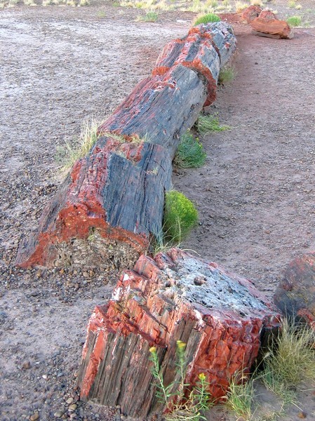
The ancient trees of Petrified Forest National Monument – preserved as quartz crystal moulds of trees buried by sediments before they decomposed – are over 200 million years old.

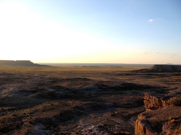
At that time, in the Late Triassic, northeastern Arizona was located near the equator resulting in a tropical climate and vegetation. The climate and landscape couldn’t be much more different now and the sheer scale of change (both time and location) are hard to comprehend looking out over the desert sunset.

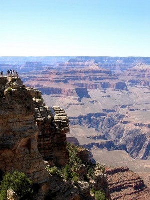
The physical size of the Grand Canyon isn’t much easier to comprehend, even when you’re stood at the very edge of the southern rim.

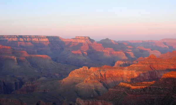
By the time the Colorado river had begun carving the canyon a mere 17 million years ago, the processes leading to its formation had already been at work for around 2,000 million years (the lowest sediments at the bottom of the Inner Gorge date to around that time). Sunset here is no less timeless than in the Petrified Forest.

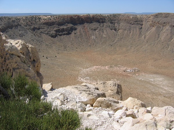
Compared with the forest and the gorge the Barringer Crater was created in the blink of an eye. But the 300,000 ton meteor that hit earth 50,000 years ago had probably being travelling on that collision course for a much longer time.

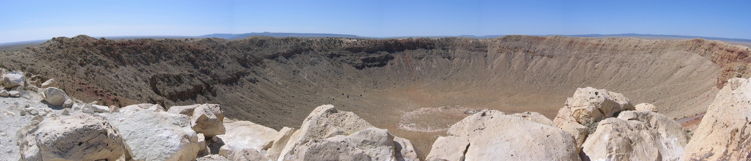
That these awesome features remain – so huge in time and space – reminds us how fleeting our biological landscapes are.

Disturbance and Landscape Dynamics in a Changing World

Experimentation can be tricky for landscape ecologists, especially if we’re considering landscapes at the human scale (it’s a bit easier at the beetle scale [pdf]). The logistic constraints of studies at large spatial and temporal scales mean we frequently use models and modelling. However, every-now-and-then certain events afford us the opportunity for a ‘natural experiment’ – situations that are not controlled by an experimenter but approximate controlled experimental conditions. In her opening plenary at ESA 2009, Prof. Monica Turner used one such natural experiment – the Yellowstone fires of 1988 – as an exemple to discuss how disturbance affects landscape dynamics and ecosystem processes. Although this is a great example for landscapes with limited human activity, it is not such a useful tool for considering human-dominated landscapes.


Landsat satellite image of the Yellowstone fires on 23rd August 1988. The image is approximately 50 miles (80 km) across and shows light from the green, short-wave infrared, and near infrared bands of the spectrum. The fires glow bright pink, recently burned land is dark red, and smoke is light blue.

Before getting into the details, one of the first things Turner did was to define disturbance (drawing largely on Pickett and White) and an idea that she views as critical to landscape dynamics – the shifting mosaic steady state. The shifting mosaic steady state, as described by Borman and Likens, is a product of the processes of vegetation disturbance and succession. Although these processes mean that vegetation will change through time at individual points, when measured over a larger area the proportion of the landscape in each seral stage (of succession) remains relatively constant. Consequently, over large areas and long time intervals the landscape can be considered to be in equilibrium (but this isn’t necessarily always the case).

Other key ideas Turner emphasised were:

  • disturbance is a key component in ecosystems across many scales,
  • disturbance regimes are changing rapidly but the effects are difficult to predict,
  • disturbance and heterogeneity have reciprocal effects.

Landscape Dynamics
In contrast to what you might expect, very large disturbances generally increase landscape heterogeneity. For example, the 1988 Yellowstone fires burned 1/3 of the park in all forest types and ages but burn severity varied spatially. Turner highlighted that environmental thresholds may determine whether landscape pattern constrains fire spread. For instance, in very dry years spatial pattern will likely have less effect than years where rainfall has produced greater spatial variation in fuel conditions.

Turner and her colleagues have also found that burn severity, patch size and geographic location affected early succession in the years following the Yellowstone fires. Lodgepole pine regeneration varied enormously across the burned landscape because of the spatial variation in serotiny and burn severity. Subsequently, the size, shape and configuration of disturbed patches influenced succession trajectories. Turner also highlighted that succession is generally more predictable in small patches, when disturbances are infrequent, and when disturbance severity/intensity is low (and vice versa).

Ecosystem Processes
One of the questions landscape ecologists have been using the Yellowstone fires to examine is; do post-disturbance patterns affect ecosystem processes? Net Primary Production varies a lot with tree density (e.g., density of lodgepole pine following fire) and the post-fire patterns of tree density have produced a landscape mosaic of ecosystem process rates. For example, Kashian and colleagues found spatial legacy effects of the post-fire mosaic can last for centuries. Furthermore, this spatial variation in ecosystem process rates is greater than temporal variation and the fires produced a mosaic of different functional trajectories (a ‘functional mosaic’).

Another point Turner was keen to make was that the Yellowstone fires were not the result of fire suppression as is commonly attributed, but instead they were driven by climate (particularly hot and dry conditions). Later in the presentation she used the ecosystem process examples above to argue that the Yellowstone fires were not an ecological disaster and that the ecosystem has proven resilient. However, she stressed that fire will continue to be an important disturbance and that the fire regimes is likely to change rapidly if climate does. For example, Turner highlighted the study by Westerling and colleagues that showed that increased fire activity in the western US in recent decades is a result of increasing temperatures, earlier spring snowmelt and subsequent increases in vegetation moisture deficit. If climate change projections of warming are realised, by 2100 the climate of 1988 (which was extreme) could become the norm and events like the Yellowstone fires will be much more frequent. For example, using a spatio-temporal state-space diagram (seebelow), Turner and colleagues [pdf] found that fires in Yellowstone during the 15 years previous to 1988 had relatively little impact on landscape dynamics (shown in green in the lower left of the diagram). However, the extent of the 1988 fires pushed the disturbance regime up into an area of the state-space not characteristic of a shifting-mosaic steady state (shown in red).


The spatio-temporal state-space diagram used by Turner and colleagues [pdf] to describe potential landscape disturbance dynamics. On the horizontal x-axis is the ratio of disturbance extent (area) to the landscape area and on the vertical y-axis is the ratio of disturbance interval (time) to recovery interval. Landscapes in the upper left of the diagram will appear to an observer as relatively constant in time with little disturbance impact; those in the lower right are dominated by disturbance.

Remaining Questions
Turner finished her presentation by highlighting what she sees as key questions for studying disturbance and landscape dynamics in a changing world:

  • How will disturbance interact with one another?
  • How will disturbances interact with other drivers?
  • What conditions will cause qualitative shifts in disturbance regimes (like that shown in the diagram above)?

It was comforting to hear that a leader in the field identified these points as important as many of them relate closely to what I’ve been working on thinking about. For example, the integrated ecological-economic forest modelling project I’m working on here in Michigan explicitly considers the interaction of two disturbances – human timber harvest and deer herbivory. The work I initiated during my PhD relates to the second question – how does human land use/cover change interact and drive changes in the wildfire regime of a landscape in central Spain? And recently, I reviewed a new book on threshold modelling in ecological restoration for Landscape Ecology.

Much of Turner’s presentation and discussion applied to American landscapes with limited human activity. This not surprising of course, given the context of the presentation (at the Ecological Society of America) and the location of her study areas (all in the USA). But although natural experiments like the 1988 Yellowstone fires may be useful as an analogue to understand processes and dynamics in similar systems, it is also interesting (and important) to think about how other systems potentially differ from this examplar. For example, the Yellowstone fires natural experiment has little to say about disturbance in human-dominated landscapes that are prevalent in many areas of the world (such as the Mediterranean Basin). In the future, research and models of landscape succession-disturbance dynamics will need to focus as much attention on human drivers of change as environmental drivers.

Turner concluded her plenary by emphasising that ecologists must increase their efforts to understand and anticipate the effects of changing disturbance regimes. This is important not only in the context of climate as driver of change, but also because of the influence of a growing human population.

Challenges and Opportunities in CHANS Research

The discussion forum is now up and running at CHANS-Net. I have just posted some questions regarding challenges and opportunities in CHANS research that arose from the CHANS workshop at US-IALE 2009. The topics include;

  • Abstract vs. Applied Research
  • Communication in CHANS Research
  • Conceptualizing Human-Environment Relationships
  • Pattern and Process in CHANS Research
  • Spider Diagrams
  • Future Directions for CHANS Research

Register in the CHANS-Net Forum, read the questions and post your replies there.

Accuracy 2010


I’ve mentioned uncertainty several times on this blog in the past (examples one and two), so it seems appropriate to highlight the next International Symposium on Spatial Accuracy Assessment in Natural Resources and Environmental Sciences. The ninth occurrence of this biennial meeting will be hosted by the University of Leicester, UK, 20th – 23rd July 2010. Oral presentations, posters and discussion will address topics including:

Semantic uncertainty and vagueness
Modelling uncertainty using geostatistics
Propagation of uncertainty in GIS
Visualizing spatial uncertainty
Uncertainty in Remote Sensing
Spatiotemporal uncertainty
Accuracy and uncertainty of DEMs
Modelling scale in environmental systems
Positional uncertainty

The deadline for abstract submission is 28th September 2009.

Incendio en un Paisaje Mediterráneo

Our recent paper describing and testing the Mediterranean Landscape Fire Succession Model I developed during my PhD has caught the eye of some folks in Spain. sinc (Servicio de Informacion y Noticias Cientificas), a Spanish scientific news website <a href="
http://plataformasinc.es/index.php/esl/Noticias/Un-modelo-predice-la-evolucion-del-paisaje-mediterraneo-tras-los-incendios&#8221; class=”regular”, target=”_blank”>has posted details of the paper (in Spanish) – hopefully it will generate some interest in our work and that some find it useful for their own.

Update 18th August 2009
Several other websites have picked up on the sinc summary and re-published an English version:

ESA 2009 Agenda

I’ve just arrived in Albuquerque, New Mexico, for the Ecological Society of American meeting. Before heading out to explore town I’ve been putting the final touches to my presentation (Monday, 4.40pm, Sendero Ballroom III) and working out what I’m going to do this week. Here’s what I think I’ll be doing:

i) Importantly, on Monday at 2.30 I’ll be going to support Megan Matonis as she talks about the work she’s been doing on our UP project: ‘Gap-, stand-, and landscape-scale factors affecting tree regeneration in harvest gaps’.

ii) Monday morning I think I’ll attend the special session ‘What is Sustainability Science and Can It Make Us Sustainable?’ [“What is sustainability science and can it make us sustainable? If sustainability science requires interdisciplinarity, how do these diverse disciplines integrate the insights that each brings? How do we reconcile differing basic assumptions to solve an urgent and global problem? How do we ensure that research outputs of ecology and other disciplines lead toward sustainability?”]

iii) Tuesday, amongst other things, I’ll check out the symposium entitled; ‘Global Sustainability in the Face of Uncertainty: How to More Effectively Translate Ecological Knowledge to Policy Makers, Managers, and the Public’. [“The basic nature of science, as well as life, is that there will always be uncertainty. We define uncertainty as a situation in which a decision-maker (scientist, manager, or policy maker) has neither certainty nor reasonable probability estimates available to make a decision. In ecological science we have the added burden of dealing with the inherent complexity of ecological systems. In addition, ecological systems are greatly affected by chance events, further muddying our ability to make predictions based on empirical data. Therefore, one of the most difficult aspects of translating ecological and environmental science into policy is the uncertainty that bounds the interpretation of scientific results.”]

iv) Wednesday I plan on attending the symposium ‘What Should Ecology Education Look Like in the Year 2020?’ [“How should ecology education be structured to meet the needs of the next generation, and to ensure that Americans prioritize sustainability and sound ecological stewardship in their actions? What balance between virtual and hands-on ecology should be taught in a cutting-edge ecological curriculum? How can we tackle the creation versus evolution controversy that is gaining momentum?”]

v) Being a geographer (amongst other things) on Thursday I’d like to participate in the discussion regarding place; ‘The Ecology of Place: Charting a Course for Understanding the Planet’ [“The diversity, complexity, and contingency of ecological systems both bless and challenge ecologists. They bless us with beauty and endless fascination; our subject is never boring. But they also challenge us with a difficult task: to develop general and useful understanding even though the outcomes of our studies typically depend on a host of factors unique to the focal system as well as the particular location and time of the study. Ecologists address this central methodological dilemma in various ways. … Given the pressing environmental challenges facing the planet, it is critical that ecologists develop an arsenal of effective strategies for generating knowledge useful for solving real-world problems. This symposium inaugurates discussion of one such strategy – The Ecology of Place.”]

vi) Also on Thursday I think I’ll see what’s going on in the session; ‘Transcending Tradition to Understand and Model Complex Interactions in Ecology’. [“Ecology intersects with the study of complex systems, and our toolboxes must grow to meet interdisciplinary needs.”]

vii) Not sure about Friday yet…

Ensemble Modelling

Uncertainty is an inherent part of modelling. Models by definition are simplified representations of reality – as such they are all wrong. Being wrong doesn’t necessarily make them useless, but it helps to have some idea about how wrong they are for them to be most useful. That’s why we should always try to provide some means to assess the uncertainty in our models output. Producing multiple realisations of a model and its results – a model ensemble – is one way to do this.

Depending on our model we can use ensemble methods to examine four different sources of modelling uncertainty:

a) Model Structure: how appropriate are our model variables, relationships and rules?

b) Model Parameters: what numerical values appropriately represent the strengths of relationships between variables?

c) Initial Conditions: how does our uncertainty in the initial state of the system we are modelling propagate through the model to the output?

d) Boundary Conditions: how do alternative (uncertain) scenarios of events that perturb our model influence output?

In their recent paper, Arujo and New show how ensemble modelling might be used to assess the impacts of these different kinds of uncertainty on model output. They advocate the use of multiple models within an ensemble forecasting framework and argue that more robust forecasts can be achieved via the appropriate analysis of ensemble forecasts. This is important because projections between different models can be so variable as to compromise their usefulness for guiding policy decisions. For example, upon examining nine bioclimatic models for four South African plant species, Pearson et al. found that for different scenarios of future climate predicted changes in species distribution varied from 92% loss to 322% gain between the different models! It’s uncertainty like this that stifles debate about the presence and impacts of anthropogenic climate change. Araujo and New go on to discuss the uses and limitations of ensemble modelling for supporting policy decisions in biodiversity conservation.

In a previous post I discussed how Bayesian methods can be used to examine uncertainty in model structure. I’ve been using Bayesian Model Averaging to help me identify which are the most appropriate predictors of local winter white-tailed deer density for our UP Forest project. Using the relationships developed via that modelling process I’ve produced spatial estimates of deer density in northern hardwood stands for a section of our study area (example below).


Hopefully forest managers will find this sort of modelling useful for their planning (I’ll ask them sometime). However, I think this sort of product will be even more useful if I can provide the managers with a spatial estimate of uncertainty in the deer density estimates. This is important not only to emphasise that there is uncertainty in the model results generally, but also to highlight where (in the landscape) the model is more or less likely to be correct. Here’s the uncertainty map corresponding with the deer density estimate map above.


In this map the lighter colours (yellows and greens) indicate less certainty in the deer density estimate at that point. If managers were to take action in this landscape to reduce deer densities they could use a combination of the maps to find locations where deer densities are estimated to be high with low uncertainty.

To be more specific, the uncertainty map above is the standard deviation of 1,000 deer density estimate maps (correspondingly the deer density map is the mean of these 1,000 models). For each of the 1,000 deer density estimates I used slightly different model parameter values, each chosen with a certain probability. These 1,000 realisations are my model ensemble. The probability a value would be chosen for use as a parameter in any of the 1,000 models was specified by a (normal) probability distribution which came from the mean and standard deviation provided by the original Bayesian regression model. To produce the 1,000 models and sample their parameter values from a probability distribution I wrote my own program which made use of the standalone R math libraries built by Chris Jennings.

Appropriately representing and communicating uncertainty in model output is vital if models and modelling is to be useful for non-modellers (e.g., policy-makers, natural resource managers, etc.). Spatial ensemble modelling helps us to do this by identifying locations where we are more or less confident about our model output.

Food Choices

I started thinking more closely about food – where it comes from, how it’s produced, how I might choose more sustainable foods – after hearing a keynote speech by Prof. Jon Foley at US-IALE 2009. Making the ‘right’ choice can be tricky, however. For example, there’s a difference between ‘natural’ and ‘organic’ and you need to consider a myriad of things if you want to know how much oil there is in your oatmeal. Working out which of the products on the shelves of your supermarket are most sustainable will hopefully be easier in the future if Wal-Mart successfully follows through on its plans to develop a ‘sustainability index’. In the meantime, the new movie Food Inc. may provide some motivation to think more carefully about the food we eat. I haven’t seen it yet but the trailer looks provoking.

New Models for Ecosystems Dynamics and Restoration

Recently I’ve been working on a review of the latest contribution to The Science and Practice of Ecological Restoration book series, entitled New Models for Ecosystems Dynamics and Restoration (edited by Hobbs and Suding). Here’s an outline of what I’ve been reading and thinking about – the formal review will appear in print in Landscape Ecology sometime in the future.

The Society for Ecological Restoration defines ecological restoration as an “intentional activity that initiates or accelerates the recovery of an ecosystem with respect to its health, integrity and sustainability”. Restoration ecology is a relatively young academic field of study that addresses problems faced by land managers and other restoration practitioners. Young et al. suggest that models of succession, community assembly and state transitions are an important component of ecological restoration, and that seed and recruitment limitation, soil processes and diversity-function relationships are also important.

The ‘new’ models referenced in the title of the book are ‘threshold’ or ‘regime shift’ ecosystem models. These models are ‘new’, the editors argue, in the sense that they contrast gradual continual models and stochastic models. Gradual continuous models are described as those that assume post-disturbance ecosystem recovery follows a continuous, gradual trajectory and are associated with classical, Clementsian theory that assumes steady, uni-directional change towards some single equilibrium state. Stochastic models assume exogenous drivers dominate the behavior of ecosystems to the extent that non-equilibrium and unstable systems states are the norm. Threshold models assume there are multiple (in contrast to the Clementsian view) stable (in contrast to the stochastic view) ecosystem states and represent changes from one relatively distinct system state to another as the result of small changes in environmental (driving) conditions. Thresholds and regime shifts are important to consider in restoration ecology as there may be thresholds in system states beyond which recovery to the previous (healthy) state is not possible.

Two types of threshold model are considered in New Models;

i) state-and-transition (S-T) models that represent multiple (often qualitative) stable states and the potential transitional relationships between those states (including the rates of transition), and

ii) alternative stable state (ASS) models which are a subset of S-T models and generally represent systems with fewer states and faster transitions (flips) between the alternative states.

For example, S-T models are often used to represent vegetation and land cover dynamics (as I did in the LFSM I developed to examine Mediterranean landscape dynamics), whereas ASS models are more frequently used for aquatic systems (e.g. lake ecosystems) and chemical/nutrient dynamics.

New Models focuses on use of these models in ecological restoration and provides an excellent introduction to key concepts and approaches in this field. Two of the six background chapters in this introduction address models and inference, two introduce transition theory and dynamics in lake and terrestrial ecosystems (respectively), and two discuss issues in social-ecological and rangeland systems. These background chapters are clear and concise, providing accessible and cogent introductions to the systems concepts that arise in the later case studies. The case studies present research and practical examples of threshold models in a range of ecosystems types – from arid, grassland, woodland and savanna ecosystems, though forest and wetland ecosystems, to ‘production landscapes’ (e.g. restoration following mining activities). Although the case study chapters are interesting examples of the current state of the use and practice of threshold modeling for ecological restoration, from my perspective there are certain issues that are insufficiently addressed. Notably, there is limited explicit consideration of spatial interactions or feedbacks between social and ecological systems.

For example, in their background chapter King and Whisenant highlight that many previous studies of thresholds in social-ecological systems have investigated an ecological system driven by a social system, ignoring feedbacks to the social components. Explicitly representing the links between social and ecological components in models does remain a daunting task, and many of the case studies continue in the same vein as the ‘uni-directional’ models King and Whisenant hint at (and I’ve discussed previously). The editors themselves highlight that detailed consideration of social systems is beyond the scope of the book and that such issues are addressed elsewhere (including in other volumes of the Ecological Restoration book series – Aronson et al.). However, representing human-environment feedbacks is becoming increasingly vital to ensure appropriate understanding of many environmental systems and their omission here may prove unsatisfactory to some.

A second shortcoming of the book, from the perspective of a landscape ecologist, is the general lack of consideration for spatial pattern and scaling and their influences on the processes considered in the case studies. In their background chapter on resilience theory and rangelands, Bestelmeyer et al. do highlight the importance of a landscape perspective and considering land as being a ‘state mosaic’, but only a single case study really picks up on these concepts in earnest (Cale and Willoughby). Other case studies do indirectly consider spatial feedbacks and landscape context, but explicit representation of relationships between spatial patterns and ecosystems processes is lacking.

However, these criticisms do need to be considered in light of the objectives of New Models. At the outset, the editors state that the book aims to collectively evaluate threshold modeling approaches as applied to ecological restoration – to examine when and where these models have been used, what evidence is used to derive and apply them, and how effective they are for guiding management. In their synthesis chapter the editors highlight that the models presented in the book have been used heuristically with little testing of their assumptions and ask; “Does this indicate an obvious gap between ecological theory and restoration practice?” For example, in their chapter on conceptual models for Australian wetlands, Sim et al. argue that the primary value of threshold models is to provide a conceptual framework of how ecosystems function relative to a variety of controlling variables. The editors’ suggestion is that restoration practitioners are applying models that work rather than “striving to prove particular elements” (of system function or ecological theory), and that maybe this isn’t such a bad approach given pressing environmental problems.

Potentially, this is a lesson that if landscape ecologists are to provide ecosystem managers and stewards with timely advice they may need to need to scale-back (i.e., reduce the complexity of) their modeling aims and objectives. Alternatively, we could view this situation as an opportunity for landscape ecologists to usefully contribute to advance the field of ecological restoration. Most likely it is indicative that where practical knowledge is needed quickly, simple models using established ecological theory and modelling tools are most useful. But in time, as our theoretical understanding and representation of spatial and human-environment interactions advances, these aspects will be integrated more readily into practical applications of modelling for ecological restoration.

Buy at Amazon

Bayesian Multimodel Inference

The abstract we submitted to the ESA Meeting was accepted a while back. Since we submitted it, Megan and I have been back in the field for some additional data collection and I’ve been doing some new analyses. Some of these new analyses are the result of my attendance at the Bayesian statistics workshop at US-IALE in Snowbird. Since then I’ve been learning more by picking the brain of a former advisor, George Perry, and doing a fair bit of reading (reading list with links at bottom). And of course, using my own data has helped a lot.

One of the main questions I’m facing, as many ecologists often do, is “which variables should be in my regression model?” This question lies at the core of model inference and assumes that it is appropriate to infer ecological process from data by searching for the single model that represents reality most accurately. However, as Link and Barker put it:

“It would be nice if there were no uncertainty about models. In such an ideal world, a single model would be available; the data analyst would be in the enviable position of having only to choose the best method for fitting model parameters based on the available data. The choice would be completely determined by the statistician’s theory, a theory which regards the model as exact depiction of the process that generated the data.

“It is clearly wrong to use the data to choose a model and then to conduct subsequent inference as though the selected model were chosen a priori: to do so is to fail to acknowledge the uncertainties present in the model selection process, and to incestuously use the data for two purposes.”

Thus, it usually more appropriate to undertake a process of multi-model inference and search for the ‘best’ possible model (given current data) rather than a single ‘true’ model. I’ve been looking into the use of Bayesian Model Averaging to address this issue. Bayesian approaches take prior knowledge (i.e., a probability distribution) and data about a system and combine them with a model to produce posterior knowledge (i.e., another probability distribution). This approach differs from the frequentist approach to statistics which calculates probabilities based on the idea of a (hypothetical) long-run of outcomes from a sequence of repeated experiments.

For example, estimating the parameters of a linear regression model using a Bayesian approach differs from a frequentist ordinary least squares (OLS) approach in two ways:

i) a Bayesian approach considers the parameter to be a random variable that might take a range of values each with a given probability, rather than being fixed with unknown probability,

ii) a Bayesian approach conditions the parameter estimate probability on the sample data at hand and not as the result of a set of multiple hypothetical independent samples (as the OLS approach does).

If there is little prior information available about the phenomena being modelled, ‘uninformative priors’ (e.g., a normal distribution with a relatively large variance about a mean of zero) can be used. In this case, the parameter estimates produced by the Bayesian linear regression will be very similar to those produced by regular OLS regression. The difference is in the error estimates and what they represent; a 95% confidence interval produced by a Bayesian analysis specifies that there is a 95% chance that the true value is within that interval given the data analyzed, whereas a 95% confidence interval from a frequentist (OLS) approach implies that if (hypothetical) data were sampled a large number of times, the parameter estimate for those samples would lie within that interval 95% of those times.

There has been debate recently in ecological circles about the merits of Bayesian versus frequentist approaches. Whilst some have strongly advocated the use of Bayesian approaches (e.g., McCarthy 2007), others have suggested a more pluralistic approach (e.g., Stephens et al. 2005). One of the main concerns with the approach of frequentist statistics is related to a broader criticism of the abuse and misuse of the P-value. For example, in linear regression models P-values are often used to examine the hypothesis that the slope of a regression line is not equal to zero (by rejecting the null hypothesis that is equal to zero). Because the slope of a regression line on a two-dimensional plot indicates the rate of change of one measure with respect to the other, a non-zero slope indicates that as one measure changes, so does the other. Consequently it is often inferred that a processes represented by one measure had an effect, or caused, the change in the other). However, as Ben Bolker points out in his excellent book:

“…common sense tells us that the null hypothesis must be false, because [the slope] can’t be exactly zero [due to the inherent variation and error in our data] — which makes the p value into a statement about whether we have enough data to detect a non-zero slope, rather than about whether the slope is actually different from zero.”

This is not to say there’s isn’t a place for null hypothesis testing using P-values in the frequentist approach. As Stephens et al. argue, “marginalizing the use of null-hypothesis testing, ecologists risk rejecting a powerful, informative and well-established analytical tool.” To the pragmatist, using whatever (statistical) tool available seems eminently more sensible than placing all one’s eggs in one basket. The important point is to try to make sure that the hypotheses one tests with P-values are ecologically meaningful.

Back to Bayesian Model Averaging (BMA). BMA provides a method to account for uncertainty in model structure by calculating (approximate) posterior probabilities for each possible model (i.e., combination of variables) that could be constructed from a set of independent variables (see Adrian Raftery’s webpage for details and examples of BMA implementation). The ‘model set’ is all possible combinations of variables (equal to 2n models, where n is the number of variables in the set). The important thing to remember with these probabilities is that it is the probability that the model is the best one from the model set considered – the probability of other models with variables not measured or included in the model set obviously can’t be calculated.

The advantage over other model selection procedures like stepwise regression is that the output provides a measure of the performance of many models, rather than simply providing the single ‘best’ model. For example, here’s a figure I derived from the output BMA provides:

The figure shows BMA results for the five models with highest posterior probability of being the best candidate model from a hypothetical model set. The probability that each model is the best in the model set is shown at top for each model – Model 1 has almost 23% chance that it is the best model given the data available. Dark blocks indicate the corresponding variable (row) is included in a given model – so Model 1 contains variables A and B, whereas Model 2 contains Variable A only. Posterior probabilities of variables being included in the best model (in the model set) are shown to the right of the blocks – as we might expect given that Variable A is present in the five most probable models it has the highest chance of being included in the best model. Click for a larger image.

BMA also provides a posterior probability for each variable being included in the best candidate model. One of the cool things about the variable posterior probability is that it can be used to produce a weighted mean value from all the models for each variable parameter estimate, each with their own Bayesian confidence interval. The weight for each parameter estimate is the probability that variable is present in the ‘best’ model. Thus, the ‘average’ model accounts for uncertainty in variable selection in the best candidate model in the individual parameter estimates.

I’ve been using these approaches to investigate the potential factors influencing local winter white-tailed deer density in in managed forests of Michigan’s Upper Peninsula. One of the most frequently used, and freely available, software packages for Bayesian statistics is WinBUGS. However, because I like to use R I’ve been exploring the packages available in that statistical language environment. Specifically, the BRugs package makes use of many OpenBUGS components (you actually provide R with a script in WinBUGS format to run) and the BMA package provides functionality for model averaging. We’re in the final stages of writing a manuscript incorporating these analyses – once it’s a bit more polished (and submitted) I’ll provide an abstract.

Reading List
Model Inference: Burnham and Anderson 2002, Stephens et al. 2005, Link and Barker 2006, Stephens et al. 2007

Introduction to Bayesian Statistics: Bolker 2007 [webpage with chapter pre-prints and exercises here], McCarthy 2007

Discussion of BMA methods: Hoeting et al. 1999, Adrian Raftery’s Webpage

Examples of BMA application: Wintle et al. 2003, Thomson et al. 2007

Criticisms of Stepwise Regression: James and McCulloch 1990, Whittingham et al. 2006