Seeds and Quadtrees

The main reason I haven’t blogged much recently is because all my spare time has been taken up working on revisions to a paper submitted to Environmental Modelling and Software. Provisionally entitled ‘Modelling Mediterranean Landscape Succession-Disturbance Dynamics: A Landscape Fire-Succession Model’, the paper describes the biophysical component of the coupled human-natural systems model I started developing during my PhD studies. This biophysical component is a vegetation state-and-transition model combined with a cellular-automata to represent wildfire ignition and spread.

The reviewers of the paper wanted to see some changes to the seed dispersal mechanism in the model. Greene et al. compared three commonly used empirical seed dispersal functions and concluded that the log-normal distribution is generally the most suitable approximation to observed seed dispersal curves. However, dispersal functions using an exponential function have also been used. A good example is the LANDIS forest landscape simulation model that calculates the probability of seed fall (P) in a region between the effective (ED) and maximum (MD) seed distance from the seed source. For distances from the seed source (x) < ED, P = 0.95. For x > MD, P = 0.001. For all other distances P is calculated using the negative exponential distribution function is used as follows:
where b is a shape parameter.

Recently Syphard et al. modified LANDIS for use in the Mediterranean Type Environment of California. The two predominant pine species in our study area in the Mediterran Basin have different seed types: one (Pinus pinaster) has has wings and can fly large distances (~1km), but the other (Pinus pinea) does not. In this case a negative exponential distribution is most appropriate. However, research on the dispersal of acorns (from Quercus ilex) found that the distance distribution of acorns was best modeled by a log-normal distribution. I am currently experimenting with these two alternative seed dispersal distributions and comparing them with spatially random seed dispersal (dependent upon quantity but not locations of seed sources).

The main thing that has kept me occupied the last couple of weeks has been the implementation of these approaches in a manner that is computationally feasible. I need to run and test my model over several hundred (annual) timesteps for a landscape grid of data ~1,000,000 pixels. Keeping computation time down so that model execution does not take hundreds of hours is clearly important if sufficient model executions are to be run to ensure some form of statistical testing is possible. A brute-force iteration method was clearly not the best approach.

One of my co-authors suggested I look into the use of Quadtrees. Quadtrees are a tree data structure that are often used to partition a two dimensional space by recursively subdividing regions into quadrants (nodes). A region Quadtree partitions a region of interest into four equal quadrants. Each of these quadrants is subdivided into four subquadrants, each of which is subdivided and so on to the finest level of spatial resolution required. The University of Maryland have a nice Java applet example that helps illustrate the concept.

For our seed dispersal purposes, a region quadtree with n levels of may be used to represent an landscape of 2n × 2n pixels, where each pixel is assigned a value of 0 or 1 depending upon whether it contains a seed source of the given type or not. The distance of all landscape pixels to a seed source can then be quickly calculated using this data structure – staring at the top level we work our way down the tree querying whether each quadrant contains a pixel(s) that is a seed source. In this way, large areas of the grid can be discounted as not containing a seed source, thereby speeding the distance calculation.

Now that I have my QuadTree structure in place model execution time is much reduced and a reasonable number of model executions should be possible over the next month or so of model testing, calibration and use. My next steps are concerned with pinning down the appropriate values for ED and MD in the seed dispersal functions. This process of parameterization will take into account values previously used by similar models in similar situations (e.g. Syphard et al.) and empirical research and data on species found within our study area (e.g. Pons and Pausas). The key thing to keep in mind with these latter studies is their focus on the distribution of individual seeds from individual trees – the spatial resolution of my model is 30m (i.e. each pixel is 30m square). Some translation of values for individuals versus aggregated representation of individuals (in pixels) will likely be required. Hopefully, you’ll see the results in print early next year.

Shapefiles in Google Earth


Last week I put together a presentation about our Michigan UP Ecological-Economic Modeling project for our funding body. I thought it would be useful to demonstrate the location of our study area in Google Earth, so I set about learning how to import ESRI shapefiles into Google Earth. I discovered it’s really easy.

My first stop in working this out was ‘Free Geography Tools‘ and their series of posts about exporting shapefiles to Google Earth. From their list of free programs, first I tried Shp2KML by Jacob Reimers. Unfortunately this program resulted in some security conflicts with our network so I couldn’t use it. Next I tried a second program, also called shp2kml, from Zonum Solutions and that worked a treat. Zonum have several other Google Earth tools that I’ll have to try out sometime.

You can download the kml file it produced for the boundary of our study area here (right click, ‘save as’ or whatever). If you have Google Earth installed you can then just double click that file (once downloaded) and Google Earth will take you right there. When I first created the link above, I hoped that when you clicked on it the file would open automatically in Google Earth – it didn’t. But after a little playing I found that kmz files will open automatically in Google Earth. kmz files are simply zipped (compressed) kml files – I used WinRar to zip the kml file and then changed the file suffix from zip to kmz. Click here – the study area file will open automatically in Google Earth (from Firefox at least – see note below). Sweet.

I also exported shapefiles for DNR and private industrial stand boundaries which match up nicely with spatial patterns of vegetation observed in the landscape. Obviously, I can’t post these shapefiles online, but you can see evidence of land ownership boundaries in our study area right here. The light green rectangular area is non-DNR land and has been clear cut. The surrounding area is managed by the DNR (possibly selective timber harvest) – the resulting land cover from different management approaches is stark. These are the sorts of patterns and issues we will be able to examine using our ecological-economic landscape model.

[Note – When posting the presentation to our web server I also learned about MS Internet Explorer .png issues. They say they’ve fixed them, but there still seem to be some problems – try viewing this page in both IE and Firefox and note the difference (hover your cursor over the words at the bottom). Viewing the presentation pages in Firefox means the links to the .kmz files are active – they are not in IE. The issue arose becasue I used OpenOffice Impress to convert my MS PowerPoint file to html files.]

Software Add-ins for Ecological Modelling

During my modelling antics these last couple of days I seem to have been using many of the add-ins I’ve have installed with the software I use regularly. I thought I’d highlight some of them here as they are really useful tools that can expand the modelling and data manipulation possibilities of a standard software install.

Much of the modelling I do is spatial, so I’m regularly using some form of GIS. I’m most familiar with the ESRI products, but have also tinkered with things like GRASS. Two free add-ins that are really useful if you use ArcMap regularly are the Patch Analyst and Hawth’s Tools. Patch Analyst facilitates the spatial pattern analysis (making use of FRAGSTATS) of landscape patches, and the modelling of attributes associated with patches. Hawth’s Tools is an extension for ArcMap that performs a number of spatial analyses and functions that you can’t do with the standard install of ArcMap. Most of the tools are written with ecological analyses in mind, but it’s also be useful for non-ecologists with functions such as conditional point sampling, kernel density estimation and vector layer editing.

Although it is generally frowned upon for statistics (use R – see below), Microsoft Excel isn’t a bad tool for organising small and medium-sized data sets and for doing basic systems modelling (spatial simulation is a little trickier). Developed by some guys at CSIRO, Pop Tools is a free add-in for PC versions of Excel that facilitates analysis of matrix population models and the simulation of stochastic processes. It was originally written to analyse ecological models, but has been used for studies of population dynamics, financial modelling, and the calculation of bootstrap and resampling statistics. Once installed, PopTools puts a new menu item in Excel’s main menu and adds over a hundred useful worksheet functions. Regardless of whether you intend to do any modelling in Excel or not, the ASAP Utilities add-in is a must for automating many frequently required tasks (including those you didn’t even know you wanted to do in Excel!). There are selection tools (such as ‘select cell with smallest number’), text tools (such as ‘insert before current value’), information tools (such as ‘Find bad cell references (#REF!)’) and many more.

If you’re going to be doing any serious statistical analyses the current software of choice is R, the open-source language and environment for statistical computing and graphics. R provides a wide variety of statistical (linear and nonlinear modelling, classical statistical tests, time-series analysis, classification, clustering, …) and graphical techniques. If you need to analyse or manipulate large datasets R is for you – you are only restricted by the memory available on your computer. For computationally-intensive tasks, C, C++ and Fortran code can be linked and called at run time. R is also highly extensible by installing optional packages that have been written by users from around the world.

Many of the packages I use are from the Spatial and Environmetrics Task views. For example, I use spdep for calculating spatial autocorrelation, VR for computing spatial correlograms or confidence intervals for model parameters, and hier.part for hierarchical partitioning. This week I started thinking about how I will use the yaImpute package to impute the stand vegetation data we have collected at specific points in our study area across the entire landscape ready to initialise our spatial simulation model. Download the R software and the individual packages from a CRAN mirror near you.

Of course, this is just the tip of the iceberg and only a few of the most useful add-ins for the most commonly used software. For a much more complete list of more technical software and programming tools for ecological and environmental modelling see Andrea Emilio Rizzoli’s ‘Collection of Modelling and Simulation Resources on the Internet‘ or the list of Ecological Modelling links by T. Legovic’ and J. Benz.

Three New NetLogo Releases

The Center for Connected Learning and Computer-Based Modeling at Northwestern University had announced three new NetLogo releases:

4.0.2 and 3.1.5 are both bugfix releases, addressing various issues found in 4.0 and 3.1.4.

NetLogo 3D Preview 5 brings the NetLogo 3D series up to date with NetLogo 4.0.2. It includes the majority of NetLogo 4.0’s features and all of 4.0.2’s fixes.

Download these latest versions from the NetLogo homepage

Landscape Simulation Modelling

This is my fifth contribution to JustScience week.

The last couple of days I’ve discussed some techniques and case studies of statistical model of landscape processes. Monday and Tuesday I looked at the power-law frequency-area characteristics of wildfire regimes in the US, Wednesday and Thursday I looked at regression modelling for predicting and explaining land use/cover change (LUCC). The main alternative to these empirical modelling methods are simulation modelling techniques.

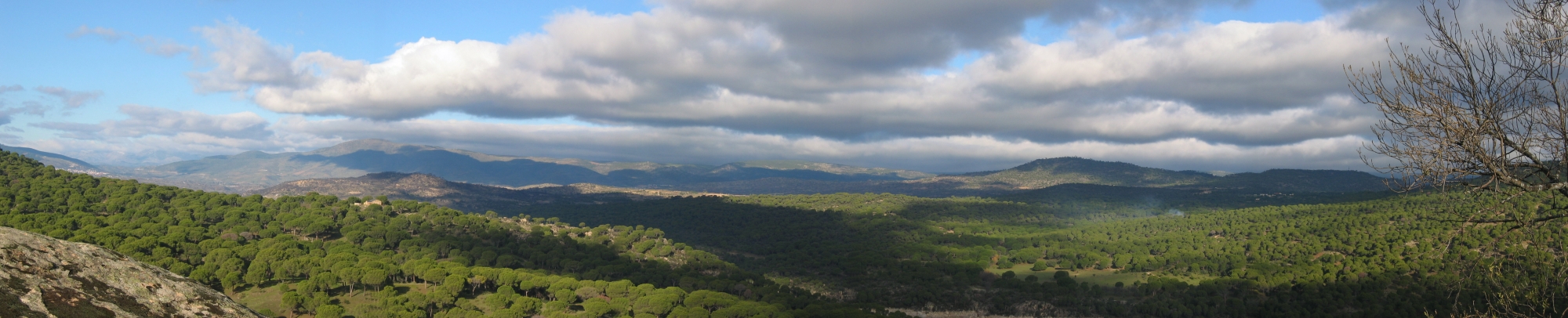
When a problem is not analytically tractable (i.e. equations cannot be written down to represent the processes) simulation models may be used to represent a system by making certain approximations and idealisations. When attempting to mimic a real world system (for example a forest ecosystem), simulation modelling has become the method of choice for many researchers. This may have become the case since simulation modelling can be used when data is sparse. Also, simulation modelling overcomes many of the problems associated with the large time and space scales involved in landscapes studies. Frequently, study areas are so large (upwards of 10 square kilometres – see photo below of my PhD study area) that empirical experimentation in the field is virtually impossible because of logistic, political and financial constraints. Experimenting with simulation models allows experiments and scenarios to be run and tested that would not be possible in real environments and landscapes.

Spatially-explicit simulation models of LUCC have been used since the 1970s and have dramatically increased in use recently with the growth in computing power available. These advances mean that simulation modelling is now one of the most powerful tools for environmental scientists investigating the interaction(s) between the environment, ecosystems and human activity. A spatially explicit model is one in which the behaviour of a single model unit of spatial representation (often a pixel or grid cell) cannot be predicted without reference to its relative location in the landscape and to neighbouring units. Current spatially-explicit simulation modelling techniques allow the spatial and temporal examination of the interaction of numerous variables, sensitivity analyses of specific variables, and projection of multiple different potential future landscapes. In turn, this allows managers and researchers to evaluate proposed alternative monitoring and management schemes, identify key drivers of change, and potentially improve understanding of the interaction(s) between variables and processes (both spatially and temporally).

Early spatially-explicit simulation models of LUCC typically considered only ecological factors. Because of the recognition that landscapes are the historical outcome of multiple complex interactions between social and natural processes, more recent spatially-explicit LUCC modelling exercises have begun to integrate both ecological and socio-economic process to examine these interactions.

A prime example of a landscape simulation model is LANDIS. LANDIS is a spatially explicit model of forest landscape dynamics and processes, representing vegetation at the species-cohort level. The model requires life-history attributes for each vegetation species modelled (e.g. age of sexual maturity, shade tolerance and effective seed-dispersal distance), along with various other environmental data (e.g. climatic, topographical and lithographic data) to classify ‘land types’ within the landscape. Previous uses of LANDIS examined the interactions between vegetation-dynamics and disturbance regimes , the effects of climate change on landscape disturbance regimes , and simulated the impacts of forest management practices such as timber harvesting.

Recently, LANDIS-II was released with a new website and a paper published in Ecological Modelling;


LANDIS-II advances forest landscape simulation modeling in many respects. Most significantly, LANDIS-II, 1) preserves the functionality of all previous LANDIS versions, 2) has flexible time steps for every process, 3) uses an advanced architecture that significantly increases collaborative potential, and 4) optionally allows for the incorporation of ecosystem processes and states (eg live biomass accumulation) at broad spatial scales.

During my PhD I’ve been developing a spatially-explicit, socio-ecological landscape simulation model. Taking a combined agent-based/cellular automata approach, it directly considers:

  1. human land management decision-making in a low-intensity Mediterranean agricultural landscape [agent-based model]
  2. landscape vegetation dynamics, including seed dispersal and disturbance (human or wildfire) [cellular automata model]
  3. the interaction between 1 and 2

Read more about it here. I’m nearly finished now, so I’ll be posting results from the model in the near future. Finally, some other useful spatial simulation modelling links:

Wisconsin Ecosystem Lab – at the University of Wisconsin

Center for Systems Integration and Sustainability – at Michigan State University

Landscape Ecology and Modelling Laboratory – at Arizona State University

Great Basin Landscape Ecology Lab – at the University of Nevada, Reno

Baltimore Ecosystem Study – at the Institute of Ecosystems Studies

The Macaulay Institute – Scottish land research centre

Volcano Modelling with Google Earth

One of my former colleagues (and good mate) at King’s, Dr. Peter Webley, is now working at The University of Alaska, Fairbanks. Pete is a volcanologist, with a particular interest in the remote monitoring and modelling of volcanic phenomena. Recently, he’s been working on the integration of Puff, a computer model of ash cloud formations, with Google Earth to improve communication between scientists and the public at large. Pretty cool stuff – checkout videos and animations here or even run your own volcano model here.

Categories: , , , ,

google maps photo page


I’ve finally got round to tidying up and completing the photos page of my website. Click on the map markers and photos taken at those locations will appear below the map. Use the links above the map to navigate. It may take a while to load first time (so be patient) and you will need JavaScript enabled in your browser.

It took a little while to get to grips with the Google Maps API, but by viewing and ‘borrowing’ code from other websites (London Satellite Photo Map was particularly helpful) I got there in the end! Go check it out! Comments? – leave them here by clicking below.

Categories: , ,

Fire-Fighting Strategy Software

Some guys at the University of Granada, Spain, have developed software for managing wildfire-fighting efforts. SIADEX is designed to speed decision-making for resource allocation, as an article in New Scientist describes:

“Computerised maps are already used by people in charge of managing the fire-fighting effort. These maps are used to plan which areas to focus on and which resources to deploy, such as fire engines, planes and helicopters.

But working out the details of such a plan involves coordinating thousands of people, hundreds of vehicles and many other resources. SIADEX is able to help by rapidly weighing up different variables.
Shift patterns

For example, it calculates which fire engines could reach an area first, where aircraft could be used, and even how to organise the shift patterns of individual fire fighters. It then very quickly produces several different detailed plans. … One plan might be the cheapest, another the fastest, and a third the least complicated.”

I wonder how Normal Maclean would have felt about this approach to fire-fighting. I imagine like me he’d be interested in how this new tool can be used to aid and protect wildland fire-fighters, but the given the unpredictability of fire behaviour (in the light of current understanding) would still maintain that human experience, gained over many years dealing with unique situations, will be invaluable in managing fire-fighters and their resources. As with much computer software, this should remain as a tool to aid human decision-making, not replace it.

Categories: , , , ,

Open-Source GIS Software

For reasons I won’t go into, I’ve had a little hassle with my laptop recently. The upshot is that I have a new machine and have been re-installing all my previous software. The one I wasn’t looking forward to was GRASS, the open-source GIS package. As I’m running windows, last time this involved installing cygwin, the Linux emulator, and installing and running it from there. A pain in the backside but I found some help online.

However, I’ve discovered that the boys and girls at GRASS have now developed a Windows native binary installation package which is A LOT easier. Follow Huidae Cho’s instructions to the letter and you’ll be just fine… What took several hours last time, took less than one this.

Other open source GIS software to check out include QGIS (using, as GRASS does, PostGIS and the PostgreSQL object-relational database) and uDig (integrable with Compendium as the guys at Econsensus have).

A longer list of useful software here.

Categories: , , , , , , , , , , , ,

dreaming code

George said it would happen. Last week I woke up one morning and realised I’d been dreaming code. I can’t say whether I was dreaming in code, or dreaming about code. Hard to tell the difference. I’m not very good at remembering what happens in my dreams – other people seem to be quite good at it though. Either way, it was a mixture of C++ and HTML. A mixture of simulation model and website I guess.

This reminded me of the title of a book that inspired a hollywood movie. “Do Androids Dream of Electric Sheep?” is apparently quite different from the movie Blade Runner, but I haven’t time for that right now so had to settle with watching the director’s cut. No time for post-modernism here (apparently the movie is, like, totally post-modern. I’ll leave Post-Normal Science to another blog) I’ll concentrate on some musings arising from my late night veiwing.

What’s the difference between a dream and a memory?” Dreams can feel immensly real, more real than memories I’d argue. They can feel so real you wake up in a cold sweat. Once you’re awake you realise it’s a dream and remember that bad dreams can happen sometimes and have happened before (but what about if you’re still asleep eh? That film Existenz). So you disregard the dream, relying on your memory that ‘it’s only a dream’. But if the dream can feel more real, why isn’t it trusted as much as the memory? Because we were unconscious when we had the dream? It wasn’t ‘real’?

So how ‘real’ are memories? What’s the relationship between the memory when it happened to the memory when it’s remembered? How has it changed? It can’t be exactly the same memory surely? I’m sure there’s a ton of literature out there on the relationship of dreams, reality, memory but I don’t know anything about that.

What I’m thinking about is the reliability of memories. We use memories to make decisions everyday. We use our memories of the past to make decisions now about the future. For someone trying to understand and simulate the decision-making process, this is quite an interesting question. Do we have some built-in understanding that sits with a memory giving us an idea about how ‘good’ (accurate) it is? If it feels vague, less vivid, if it feels less real, (if it feels less ‘real’ like a dream feels ‘real’) then this it’s not as reliable? Or is it about repetition – if we drive the same route to work everyday we remember it better than one we don’t drive often (but what about the details of that daily journey?).

Anyway, I think that’s all a little too detailed for me. It’s something interesting to think about and seemingly a popular topic for movie-makers. This guy Michel Gondry seems quite interested. Eternal Sunshine of the Spotless Mind was good – memories are more than just in your head, they’re part of you, they and the experiences that produced them make you who you are and that can’t be ignored. He’s got a new one out soon – The Science of Sleep. Looks quite fun.

I doubt it will help answer any of my questions though. I’m not going to be able to represent memories as a part of the decision-making process in my simulation model. I reckon it would be pretty ambitious for anyone to try that for a while. I’ll stick with some more general observations and mechanisms and keep dreaming code for a while longer.

[PS BAWA 1 – 3 Warmley Saints. Millington opened his scoring account in the first pre-season friendly today. A glorious 1 yard tap in, steaming in from central midfield, after the ‘keeper fumbled.]