This post is my third contribution to JustScience week.

In Land Use/Cover Change (LUCC) studies, empirical (statistical) models use the observed relationship between independent variables (for example mean annual temperature, human population density) and a dependent variable (for example land-cover type) to predict the future state of that dependent variable. The primary limitation of this approach is the inability to represent systems that are non-stationary.

Non-stationary systems are those in which the relationships between variables are changing through time. The assumption of stationarity rarely holds in landscape studies – both biophysical (e.g. climate change) and socio-economic driving forces (e.g. agricultural subsidies) are open to change. Two primary empirical models are available for studying lands cover and use change; transition matrix (Markov) models and regression models. My research has particularly focused on the latter, particularly the logistic regression model.

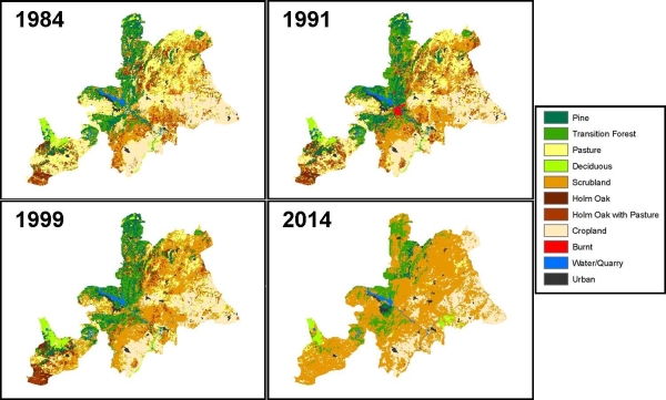
Figure 1.

Figure 1 above shows observed land cover for 3 years (1984 – 1999) for SPA 56, with a fourth map (2014) predicted from this data. Models run for observed periods of change for SPA 56 were found to have a pixel-by-pixel accuracy of up to 57%. That is, only just over half of the map was correctly predicted. Not so good really…

Pontius and colleagues have bemoaned such poor performance of models of this type, highlighting that models are often unable to perform even as well as the ‘null model of no change’. That is, assuming the landscape does not change from one point in time to another is often a better predictor of the landscape (at the second point in time) than a regression model! Clearly, maps of future land cover from these models should be understood as a projection of future land cover given observed trends continue unchanged into the future (i.e. the stationarity condition is maintained).

Acknowledgement of the stationarity assumption is perhaps more important, and more likely to be invalid, from a socio-economic perspective than biophysical. Whilst biophysical processes might be assumed to be relatively constant over decadal timescales (climatic change aside), this will likely not be the case for many socio-economic processes. With regard to SPA 56 for example, the recent expansion of the European Union to 25 countries, and the consequent likely restructuring of the Common Agricultural Policy (CAP), will lead to shifts in the political and economic forces driving LUCC in the region. The implication is that where socio-economic factors are important contributors to landscape change regression models are unlikely to be very useful for predicting future landscapes and making subsequent ecological interpretation or management decisions.

Because of the shortcomings of this type of model, alternative methods to better understanding processes of change, and likely future landscape states, will be useful. For example, hierarchical partitioning is a method for using statistical modelling in an explanatory capacity rather than for predictive purposes. Work I did on this with colleagues was recently accepted for publication by Ecosystems and I’ll discuss it in more detail tomorrow. The main thrust of my PhD however, is the development of an integrated socio-ecological simulation model that considers agricultural decision-making, vegetation dynamics and wildfire regimes.

Technorati Tag: regression, modelling, LandUse, stationarity