PhD Thesis Completed

So, finally, it is done. As I write, three copies of my PhD Thesis are being bound ready for submission tomorrow! I’ve posted a short abstract below. If you want a more complete picture of what I’ve done you can look at the Table of Contents and read the online versions of the Introduction and Discussion and Conclusions. Email me if you want a copy of the whole thesis (all 81,000 words, 277 pages of it).

So just the small matter of defending the thesis at my viva voce in May. But before that I think it’s time for a celebratory beer on the South Bank of the Thames in the evening sunshine…

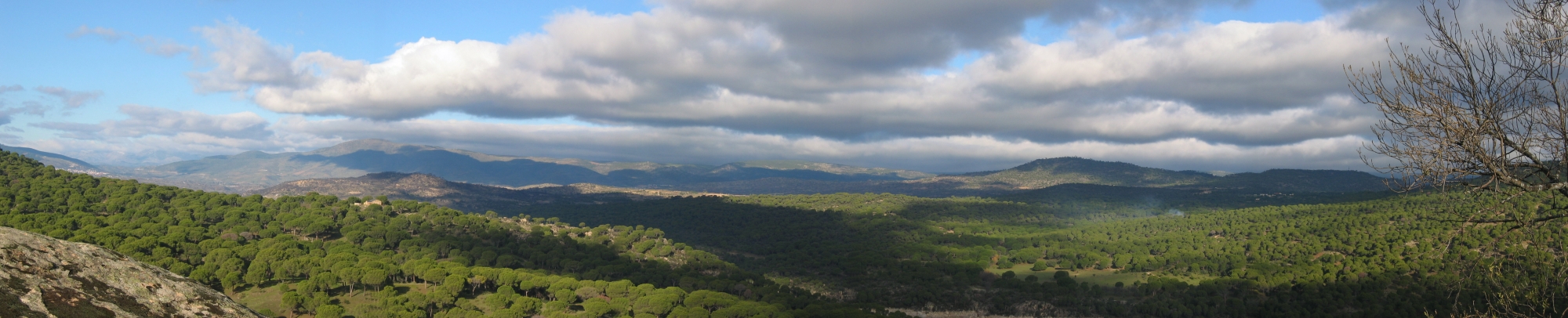
Modelling Land-Use/Cover Change and Wildfire Regimes in a Mediterranean Landscape

James D.A. Millington
March 2007

Department of Geography
King’s College, London

Abstract
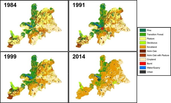
This interdisciplinary thesis examines the potential impacts of human land-use/cover change upon wildfire regimes in a Mediterranean landscape using empirical and simulation models that consider both social and ecological processes and phenomena. Such an examination is pertinent given contemporary agricultural land-use decline in some areas of the northern Mediterranean Basin due to social and economic trends, and the ecological uncertainties in the consequent feedbacks between landscape-level patterns and processes of vegetation- and wildfire-dynamics.

The shortcomings of empirical modelling of these processes are highlighted, leading to the development of an integrated socio-ecological simulation model (SESM). A grid-based landscape fire succession model is integrated with an agent-based model of agricultural land-use decision-making. The agent-based component considers non-economic alongside economic influences on actors’ land-use decision-making. The explicit representation of human influence on wildfire frequency and ignition in the model is a novel approach and highlights biases in the areas of land-covers burned according to ignition cause. Model results suggest if agricultural change (i.e. abandonment) continues as it has recently, the risk of large wildfires will increase and greater total area will be burned.

The epistemological problems of representation encountered when attempting to simulate ‘open’, middle numbered systems – as is the case for many ‘real world’ geographical and ecological systems – are discussed. Consequently, and in light of recent calls for increased engagement between science and the public, a shift in emphasis is suggested for SESMs away from establishing the truth of a model’s structure via the mimetic accuracy of its results and toward ensuring trust in a model’s results via practical adequacy. A ‘stakeholder model evaluation’ exercise is undertaken to examine this contention and to evaluate, with the intent of improving, the SESM developed in this thesis. A narrative approach is then adopted to reflect on what has been learnt.

positive thought generator

I am less than two weeks away from submitting my PhD thesis. The BBC Radio 1 Positive Thought Generator has been helping me maintain my sanity over the last few weeks…

http://www.bbc.co.uk/slink/play/games/positive/positive_gen.swf
Click the button. It’s positively uplifting.

Problems in Modelling Nature

I haven’t posted much over the last week or so – things have been super busy trying to complete my PhD thesis. I hope to be submitting the thesis in the next few weeks so there’s not likely to be much blogging going on until that’s done (and I’ve had a little rest). So until I get back something resembling a ‘normal’ routine I’ll leave you with this…

One of my advisors point out this book review in the New York Times to me. From the article it seems that in Why Environmental Scientists Can’t Predict the Future, Orrin Pilkey and Linda Pilkey-Jarvis suggest environmental models aren’t up to the job that the modellers building and using them say they are:


Dr. Pilkey and his daughter Linda Pilkey-Jarvis, a geologist in the Washington State Department of Geology, have expanded this view into an overall attack on the use of computer programs to model nature. Nature is too complex, they say, and depends on too many processes that are poorly understood or little monitored — whether the process is the feedback effects of cloud cover on global warming or the movement of grains of sand on a beach.

Their book, “Useless Arithmetic: Why Environmental Scientists Can’t Predict the Future,” originated in a seminar Dr. Pilkey organized at Duke to look into the performance of mathematical models used in coastal geology. Among other things, participants concluded that beach modelers applied too many fixed values to phenomena that actually change quite a lot. For example, “assumed average wave height,” a variable crucial for many models, assumes that all waves hit the beach in the same way, that they are all the same height and that their patterns will not change over time. But, the authors say, that’s not the way things work.

Also, modelers’ formulas may include coefficients (the authors call them “fudge factors”) to ensure that they come out right. And the modelers may not check to see whether projects performed as predicted.

Along the way, Dr. Pilkey and Ms. Pilkey-Jarvis describe and explain a host of modeling terms, including quantitative and qualitative models (models that seek to answer precise questions with more or less precise numbers, as against models that seek to discern environmental trends).

They also discuss concepts like model sensitivity — the analysis of parameters included in a model to see which ones, if changed, are most likely to change model results.

But, the authors say it is important to remember that model sensitivity assesses the parameter’s importance in the model, not necessarily in nature. If a model itself is “a poor representation of reality,” they write, “determining the sensitivity of an individual parameter in the model is a meaningless pursuit.”

Given the problems with models, should we abandon them altogether? Perhaps, the authors say. Their favored alternative seems to be adaptive management, in which policymakers may start with a model of how a given ecosystem works, but make constant observations in the field, altering their policies as conditions change. But that approach has drawbacks, among them requirements for assiduous monitoring, flexible planning and a willingness to change courses in midstream. For practical and political reasons, all are hard to achieve.

Besides, they acknowledge, people seem to have such a powerful desire to defend policies with formulas (or “fig leaves,” as the authors call them), that managers keep applying them, long after their utility has been called into question.

So the authors offer some suggestions for using models better. We could, for example, pay more attention to nature, monitoring our streams, beaches, forests or fields to accumulate information on how living things and their environments interact. That kind of data is crucial for models. Modeling should be transparent. That is, any interested person should be able to see and understand how the model works — what factors it weighs heaviest, what coefficients it includes, what phenomena it leaves out, and so on. Also, modelers should say explicitly what assumptions they make.

Some of these suggestions sounds sensible and similar to what I’ve been thinking about in my thesis. However, to suggest abandoning environmental modelling altogether – claiming that is it of no value whatsoever – seems a little excessive and I’m going reserve my judgment for now.

I’m being sent a review copy so when I get my life back I’ll take a look at it and post some more informed criticism.

Post-Normal Science (& Simulation Modelling)

Last week I didn’t quite manage to complete the JustScience week challenge to blog on a science topic, and only on science, every day that week. I managed five days but then the weekend got in the way. On those five days I wrote about the application of scientific methods to examine landscape processes – specifically wildfire regimes and land use/cover change (LUCC). Another of my ‘scientific’ interests is the relationship between science and policy- and decision-making, so what I was planning to write on Saturday might not have fitted the JustScience bill anyway. I’ll post it now instead; a brief review of some of the ways commentators have suggested science may need to adapt in the 21st century to ensure it remains relevant to ‘real world problems’.

Ulrich Beck has suggested that we now live in the ‘risk society‘. Beck’s view that the risks contemporary societies face – such as changing climates, atmospheric pollution, exposure to radioactive substances – shares common themes with others examining contemporary society and their relationships with science, technology and their environment (Giddens for example).

In the risk society, many threats are difficult to identify in everyday life, requiring complicated, expensive (usually scientific) equipment to measure and identify them. These threats, requiring methods and tools from science and technology to investigate them, have frequently been initiated by previous scientific and technological endeavours. Consequences which are no longer simply further academic and scientific problems for study, but consequences that are important socially, politically, culturally, and environmentally. Furthermore, these consequences may be imminent, potentially necessitating action before the often lengthy traditional scientific method (hypothesis testing, academic peer review etc.) has produced a consensus on the state of knowledge about it.

Beck goes on to suggest a distinction between two divergent sciences; the science of data and the science of experience. The former is older, specialised, laboratory-based science that uses the language of mathematics to explore the world. The latter will identify consequences and threats, publicly testing its objectives and standards to examine the doubts the former ignores. Traditional science, Beck suggests, is at the root of current environmental problems and will simply propagate risk further rather than reducing it.

Taking a similar perspective, Funtowicz and Ravetz have presented ‘post-normal’ science as a new type of science to replace the reductionist, analytic worldview of ‘normal’ science with a “systemic, synthetic and humanistic” approach. The term ‘post-normal’ deliberately echoes Thomas Kuhn’s formulation of ‘normal’ science functioning between paradigm shifts, to emphasise the need for a shift in scientific thinking and practices that takes it outside of the standard objective, value-free perspective. The methodology of post-normal science then, emphasises uncertainties in knowledge, quality of method, and complexities in ethics. Post-normal science, according to Funtowicz and Ravetz, embraces the uncertainties inherent in issues of risk and the environment, makes values explicit rather than presupposing them, and generates knowledge and understanding through an interactive dialogue rather than formalised deduction. You can read more about Post-Normal science itself at NUSAP.net, and the Post-Normal Times blog will keep you up-to-date on recent events and issues at the interface between science and policy-making.

Recently I’ve been thinking about the utility of environmental simulation models (particularly those that explicitly consider human activity) for examining the sorts of problems present in the ‘risk society’ and that post-normal science has been promoted as being able to contribute to. I’ll write in more detail at a later date, but briefly many of the theoretical facets post-normal science suggests seem relevant to the issues facing environmental (and landscape) simulation models. Particularly, the epistemological problems of model validation recently discussed in the academic literature (e.g. Naomi Oreskes et al., Keith Beven , and which I have touched on briefly in the past, but must post about in more detail soon) have highlighted the importance of considering the subjective aspects of the model construction process.

As a result I have come to think that model ‘validation’ might be better achieved by taking an evaluative, qualitative approach to rather than a confirmatory approach. A shift in this approach would essentially mean asking “is this model good enough” rather than “is this model true”? Ethical questions about who should be asked, and who is qualified to ask, whether a model is to be deemed trustworthy and fit for purpose to examine real world problems (and not those confined to a laboratory) also become important when these criteria are used. These model validation issues are thus resonant with a post-normal science perspective toward examining the environmental issues contemporary societies currently face.

I’ll write more on both the epistemological problems of confirmatory model validation for environmental and landscape simulation models and potential ways we might go about assessing the trustworthiness and practical adequacy of these models for addressing the problems of the ‘risk society‘ soon.

Technorati Tags: , , , , , , ,

Landscape Simulation Modelling

This is my fifth contribution to JustScience week.

The last couple of days I’ve discussed some techniques and case studies of statistical model of landscape processes. Monday and Tuesday I looked at the power-law frequency-area characteristics of wildfire regimes in the US, Wednesday and Thursday I looked at regression modelling for predicting and explaining land use/cover change (LUCC). The main alternative to these empirical modelling methods are simulation modelling techniques.

When a problem is not analytically tractable (i.e. equations cannot be written down to represent the processes) simulation models may be used to represent a system by making certain approximations and idealisations. When attempting to mimic a real world system (for example a forest ecosystem), simulation modelling has become the method of choice for many researchers. This may have become the case since simulation modelling can be used when data is sparse. Also, simulation modelling overcomes many of the problems associated with the large time and space scales involved in landscapes studies. Frequently, study areas are so large (upwards of 10 square kilometres – see photo below of my PhD study area) that empirical experimentation in the field is virtually impossible because of logistic, political and financial constraints. Experimenting with simulation models allows experiments and scenarios to be run and tested that would not be possible in real environments and landscapes.

Spatially-explicit simulation models of LUCC have been used since the 1970s and have dramatically increased in use recently with the growth in computing power available. These advances mean that simulation modelling is now one of the most powerful tools for environmental scientists investigating the interaction(s) between the environment, ecosystems and human activity. A spatially explicit model is one in which the behaviour of a single model unit of spatial representation (often a pixel or grid cell) cannot be predicted without reference to its relative location in the landscape and to neighbouring units. Current spatially-explicit simulation modelling techniques allow the spatial and temporal examination of the interaction of numerous variables, sensitivity analyses of specific variables, and projection of multiple different potential future landscapes. In turn, this allows managers and researchers to evaluate proposed alternative monitoring and management schemes, identify key drivers of change, and potentially improve understanding of the interaction(s) between variables and processes (both spatially and temporally).

Early spatially-explicit simulation models of LUCC typically considered only ecological factors. Because of the recognition that landscapes are the historical outcome of multiple complex interactions between social and natural processes, more recent spatially-explicit LUCC modelling exercises have begun to integrate both ecological and socio-economic process to examine these interactions.

A prime example of a landscape simulation model is LANDIS. LANDIS is a spatially explicit model of forest landscape dynamics and processes, representing vegetation at the species-cohort level. The model requires life-history attributes for each vegetation species modelled (e.g. age of sexual maturity, shade tolerance and effective seed-dispersal distance), along with various other environmental data (e.g. climatic, topographical and lithographic data) to classify ‘land types’ within the landscape. Previous uses of LANDIS examined the interactions between vegetation-dynamics and disturbance regimes , the effects of climate change on landscape disturbance regimes , and simulated the impacts of forest management practices such as timber harvesting.

Recently, LANDIS-II was released with a new website and a paper published in Ecological Modelling;


LANDIS-II advances forest landscape simulation modeling in many respects. Most significantly, LANDIS-II, 1) preserves the functionality of all previous LANDIS versions, 2) has flexible time steps for every process, 3) uses an advanced architecture that significantly increases collaborative potential, and 4) optionally allows for the incorporation of ecosystem processes and states (eg live biomass accumulation) at broad spatial scales.

During my PhD I’ve been developing a spatially-explicit, socio-ecological landscape simulation model. Taking a combined agent-based/cellular automata approach, it directly considers:

  1. human land management decision-making in a low-intensity Mediterranean agricultural landscape [agent-based model]
  2. landscape vegetation dynamics, including seed dispersal and disturbance (human or wildfire) [cellular automata model]
  3. the interaction between 1 and 2

Read more about it here. I’m nearly finished now, so I’ll be posting results from the model in the near future. Finally, some other useful spatial simulation modelling links:

Wisconsin Ecosystem Lab – at the University of Wisconsin

Center for Systems Integration and Sustainability – at Michigan State University

Landscape Ecology and Modelling Laboratory – at Arizona State University

Great Basin Landscape Ecology Lab – at the University of Nevada, Reno

Baltimore Ecosystem Study – at the Institute of Ecosystems Studies

The Macaulay Institute – Scottish land research centre

Hierarchical Partitioning for Understanding LUCC

This post is my fourth contribution to JustScience week.

Multiple regression is an empirical, data-driven approach for modelling the response of a single (dependent) variable from a suite of predictor (independent) variables. Mac Nally (2002) suggests that multiple regression is generally used for two purposes by ecologists and biologists; 1) to assess the amount of variance exhibited by the dependent variable that can be attributed to each predictor variable, and 2) to find the ‘best’ predictive model (the model that explains most total variance). Yesterday I discussed the use of logistic regression (a form of multiple regression) models for predictive purposes in Land Use/Cover Change (LUCC) studies. Today I’ll present some work on an explanatory use of these methods.

Finding a multivariate model that uses the ‘best’ set of predictors does not imply that those predictors will remain the ‘best’ when used independently of one another. Multi-collinearity between predictor variables means that the use of the ‘best’ subset of variables (i.e. model) to infer causality between independent and dependent variables provides little valid ‘explanatory power’ (Mac Nally, 2002). The individual coefficients of a multiple regression model can only be interpreted for direct effects on the response variable when the other predictor variables are held constant (James & McCulloch, 1990). The use of a model to explain versus its use to predict must therefore be considered (Mac Nally, 2000).

Hierarchical partitioning (HP) is a statistical method that provides explanatory power, rather than predictive. It allows the contribution of each predictor to the total explained variance of a model, both independently and in conjunction with the other predictors, to be calculated for all possible candidate models. The use of the HP method developed by Chevan and Sutherland (1991) by ecologists and biologists in their multivariate analyses was first suggested by Mac Nally (1996). More recently, the method has been extended to help provide the ability to statistically choose which variables to retain once they have been ranked for their predictive use (Mac Nally, 2002). Details of how HP works can be found here.

With colleagues, I examined the use of hierarchical partitioning for understanding LUCC in my PhD study area, leading to a recent publication in Ecosystems. We examined the difference in using two different land-cover (LC) classifications for the same landscape, one classification with 10 LC classes, another with four. Using HP we found that more coarse LC classifications (i.e. fewer LC classes) causes the joint effects of variables to suppress total variance explained in LUCC. That is, the combined effect of explanatory variables increases the total explained variance (in LUCC) in regression models using the 10-class LC classification, but reduces total explained variance in the dependent variable for four-class models.

We suggested that (in our case at least) this was because the aggregated nature of the four-class models means broad observed changes (for example from agricultural land to forested land) masks specific changes within the classes (for example from pasture to pine forest or from arable land to oak forest). These specific transitions may have explanatory variables (causes) that oppose one another for the different specific transitions, decreasing the explanatory power of models that use both variables to explain a single broader shift. By considering more specific transitions, the utility of HP for elucidating important causal factors will increase.

We concluded that a systematic examination of specific LUCC transitions is important for elucidating drivers of change, and is one that has been under-used in the literature. Specifically, we suggested hierarchical partitioning should be useful for assessing the importance of causal mechanisms in LUCC studies in many regions around the world.

Technorati Tags: , ,

Logistic Regression for LUCC Modelling

This post is my third contribution to JustScience week.

In Land Use/Cover Change (LUCC) studies, empirical (statistical) models use the observed relationship between independent variables (for example mean annual temperature, human population density) and a dependent variable (for example land-cover type) to predict the future state of that dependent variable. The primary limitation of this approach is the inability to represent systems that are non-stationary.

Non-stationary systems are those in which the relationships between variables are changing through time. The assumption of stationarity rarely holds in landscape studies – both biophysical (e.g. climate change) and socio-economic driving forces (e.g. agricultural subsidies) are open to change. Two primary empirical models are available for studying lands cover and use change; transition matrix (Markov) models and regression models. My research has particularly focused on the latter, particularly the logistic regression model.


Figure 1.

Figure 1 above shows observed land cover for 3 years (1984 – 1999) for SPA 56, with a fourth map (2014) predicted from this data. Models run for observed periods of change for SPA 56 were found to have a pixel-by-pixel accuracy of up to 57%. That is, only just over half of the map was correctly predicted. Not so good really…

Pontius and colleagues have bemoaned such poor performance of models of this type, highlighting that models are often unable to perform even as well as the ‘null model of no change’. That is, assuming the landscape does not change from one point in time to another is often a better predictor of the landscape (at the second point in time) than a regression model! Clearly, maps of future land cover from these models should be understood as a projection of future land cover given observed trends continue unchanged into the future (i.e. the stationarity condition is maintained).

Acknowledgement of the stationarity assumption is perhaps more important, and more likely to be invalid, from a socio-economic perspective than biophysical. Whilst biophysical processes might be assumed to be relatively constant over decadal timescales (climatic change aside), this will likely not be the case for many socio-economic processes. With regard to SPA 56 for example, the recent expansion of the European Union to 25 countries, and the consequent likely restructuring of the Common Agricultural Policy (CAP), will lead to shifts in the political and economic forces driving LUCC in the region. The implication is that where socio-economic factors are important contributors to landscape change regression models are unlikely to be very useful for predicting future landscapes and making subsequent ecological interpretation or management decisions.

Because of the shortcomings of this type of model, alternative methods to better understanding processes of change, and likely future landscape states, will be useful. For example, hierarchical partitioning is a method for using statistical modelling in an explanatory capacity rather than for predictive purposes. Work I did on this with colleagues was recently accepted for publication by Ecosystems and I’ll discuss it in more detail tomorrow. The main thrust of my PhD however, is the development of an integrated socio-ecological simulation model that considers agricultural decision-making, vegetation dynamics and wildfire regimes.

Technorati Tag: , , ,

Characterizing wildfire regimes in the United States

This post is my second contribution to JustScience week, and follows on from the first post yesterday.

During my Master’s Thesis I worked with Dr. Bruce Malamud to examine wildfire frequency-area statistics and their ecological and anthropogenic drivers. Work resulting from this thesis led to the publication of Malamud et al. 2005

We examined wildfires statistics for the conterminous United States (U.S.) in a spatially and temporally explicit manner. Using a high-resolution data set of 88,916 U.S. Department of Agriculture Forest Service wildfires over the time period 1970-2000 to consider wildfire occurrence as a function of biophysical landscape characteristics. We used Bailey’s ecoregions as shown by Figure 1A below.

Figure 1.

In Bailey’s classification, the conterminous U.S. is divided into ecoregion divisions according to common characteristics of climate, vegetation, and soils. Mountainous areas within specific divisions are also classified. In the paper, we used ecoregion divisions to geographically subdivide the wildfire database for statistical analyses as a function of ecoregion division. Figure 1B above shows the location of USFS lands in the conterminous U.S.

We found that wildfires exhibit robust frequency-area power-law behaviour in the 18 different ecoregions and used power-law exponents (normalized by ecoregion area and the temporal extent of the wildfire database) to compare the scaling of wildfire-burned areas between ecoregions. Normalizing the relationships allowed us to map the frequency-area relationships, as shown in Figure 2A below.

Figure 2.

This mapping exercise shows a systematic change east-to-west gradient in power-law exponent beta values. This gradient suggests that the ratio of the number of large to small wildfires decreases from east to west across the conterminous U.S. Controls on the wildfire regime (for example, climate and fuels) vary temporally, spatially, and at different scales, so it is difficult to attribute specific causes to this east-to-west gradient. We suggested that the reduced contribution of large wildfires to total burned area in eastern ecoregion divisions might be due to greater human population densities that have increased forest fragmentation compared with western ecoregions. Alternatively, the gradient may have natural drivers, with climate and vegetation producing conditions more conducive to large wildfires in some ecoregions compared with others.

Finally, this method allowed us to calculate recurrence intervals for wildfires of a given burned area or larger for each ecoregion (Figure 2B above). In turn this allowed for the classification of wildfire regimes for probabilistic hazard estimation in the same vein as is now used for earthquakes.

Read the full paper here.

Technorati Tags: , , , ,

Wildfire Frequency-Area Scaling Relationships

This post is the first of my contribution to JustScience week.

Wildfire is considered an integral component of ecosystem functioning, but often comes into conflict with human interests. Thus, understanding and managing relationship between wildfire, ecology and human activity is of particular interest to both ecologists and wildfire managers. Quantifying the wildfire regime is useful in this regard. The wildfire regime is the name given to the combination of the timing, frequency and magnitude of all fires in a region. The relationship between the frequency and magnitude of fires, the frequency-area distribution, is one particular aspect of the wildfire regime that has become of interest recently.

Malamud et al. 1998 examined ‘Forest Fire Cellular Automata‘ finding a power-law relationship between the frequency and size of events. The power-law relationship takes the form:

power-law function

where frequency is the frequency of fires with size area, and beta is a constant. beta is a measure of the ratio of small to medium to large size fires and how frequently they occur. The smaller the value of beta, the greater the contribution of large fires (compared to smaller fires) to the total burned area of a region. The greater the value, the smaller the contribution. Such a power-law relation is represented on a log-log plot as straight line, as the example from Malamud et al. 2005 shows:

power-law distribution

Shown circles are number of wildfires per “unit bin” of 1 km^2 (in this case normalized by database length in years and area in km^2) plotted as a function of wildfire area. Also shown is a solid line (best least-squares fit) with coefficient of determination r^2. Dashed lines represent lower/upper 95% confidence intervals, calculated from the standard error. Horizontal error bars on burned area are due to measurement and size binning of individual wildfires. Vertical error bars represent two standard deviations of the normalized frequency densities and are approximately the same as the lower and upper 95% confidence interval.

As a result of their work on the forest fire cellular automata Malamud et al. 1998 wondered whether the same relation would hold for empirical wildfire data. They found the power-law relationship did indeed hold for observed wildfire data for parts of the US and Australia. As Millington et al. 2006 discuss, since this seminal publication several other studies have suggested a power-law relationship is the best descriptor of the frequency-size distribution of wildfires around the world.

During my Master’s Thesis I worked with Dr. Bruce Malamud to examine wildfire frequency-area statistics and their ecological and anthropogenic drivers. Work resulting from this thesis led to the publication of Malamud et al. 2005 which I’ll discuss in more detail tomorrow.

Technorati Tags: , , ,

Adaption not Mitigation

There’s a lot written about climate change on web 2.0 – and there’s about to be a lot more written about it over the coming weeks. The impending release of the Intergovernmental Panel on Climate Change (IPCC) 4th Assessment Report is going to have plenty for the commentators and bloggers to chew on. If you were so inclined it would take you quite a while to get through it all. But if there is one thing I think you should read about climate change in the light of the latest IPCC report it’s Maragret Wente’s piece (re)posted on Seeker.

The important point raised is that although much gets written about climate change mitigation, it is at the expense of discussion about climate change adaptation.

This is not a new point – Rayner and Malone wrote about it in Nature a decade ago, and I even got the message in my third year undergrad climate modelling course. Although reducing carbon emissions is important it may not halt what has already started, and we would do well to get thinking about the best adaptation strategies to the consequences of a changing climate. Of course, we should continue working to reduce our carbon emissions. But we need to accept that, regardless of whether the change is human induced or not, in all probability the climate is changing and we need to be prepared for the consequences.

I’ve posted what I think is the more relevant section below, but the whole thing is very interesting: read the whole article;


The climate debate focuses almost entirely on mitigation (how we can slow down global warming). But climate scientists and policy experts say that in the short term — our lifetimes — our most important insurance policy is adaptation. Nothing we do to cut emissions will reduce the risk from hurricanes or rising seas in the short term. But there are other ways to reduce the risk. We can build storm-surge defences, stop building in coastal areas and make sure we protect our fresh-water supplies from salination. We also can develop crops that will do well in hotter climates.

‘Adaptation’ is not a word that figures much in climate-change debates. Activists (and much of the general public) think it sounds lazy and defeatist. But the experts talk about adaptation all the time.

Technorati Tags: , , , , ,