It’s been a while since I posted here about the forest modelling I’ve been working on here at MSU. Over the last couple of months I’ve been working on finalizing the regeneration modelling component, refining the timber harvest rules, linking simulations to the bird occupancy modelling I started this spring, and writing it all up for manuscripts.
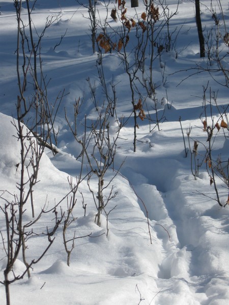
Across our study area we’ve found that regeneration of juvenile trees following timber harvest varies greatly. For example, from our empirical data we find that sugar maple saplings were present in over 70% of northern forest gaps but were completely absent from 96% of gaps in southern areas. Megan Matonis suggested in her thesis that this variation is related to snow depth, deer density and soil nutrient conditions. To examine the potential long-term effects of these differences in regeneration on forest structure I’ve been running our simulation model with pre-set levels of regeneration that reflect our observations, ranging from the maximum possible (given the space available in a post-harvest gap) to a complete absence of regenerating juvenile trees.
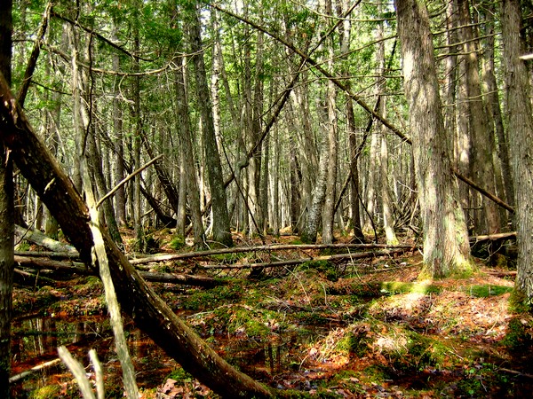
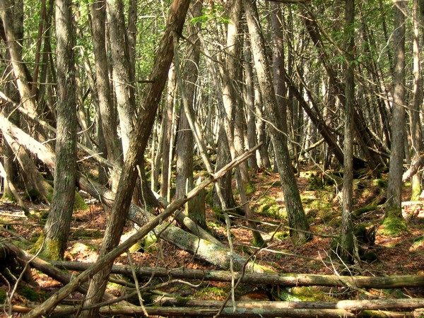
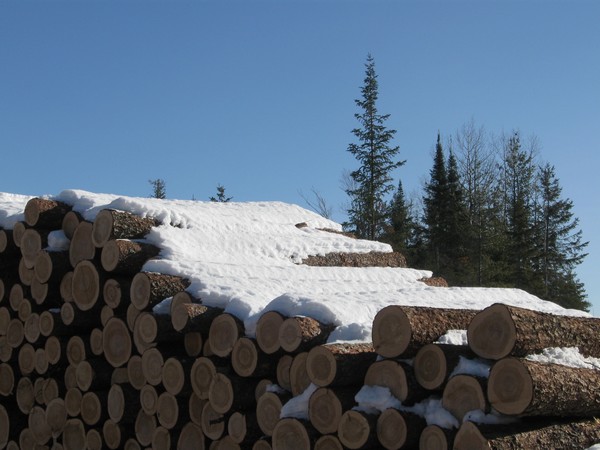
These ‘gaps’ I’m talking about are created in northern hardwood forests when individual or small groups of trees are removed in an uneven-aged timber management approach. The removal of these trees creates openings (‘gaps’) in the forest canopy allowing light into lower levels for younger trees [gaps may also be created naturally but we’re focusing on those created by human activity which is the dominant driver in our study area]. When harvesting trees in this approach foresters aim to produce a forest structure with a ‘reverse-J’ distribution of tree sizes; high densities of small, young trees and low densities of larger, older trees (approximating a gamma-distribution like I found in our data previously). The idea is that through time an abundant supply of competing smaller trees will replace larger trees trees that are removed.
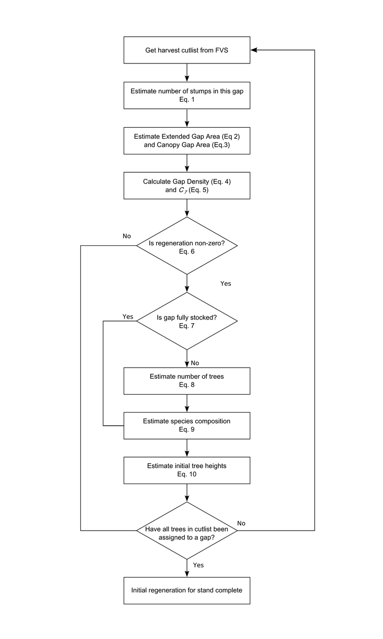
Representing this approach in our model (using FVS keywords [.pdf]) requires quite a bit of code, but working through the example provided by Don Vandendriesche [.pdf] helped. This approach requires the model user to specify a residual basal area (the area occupied by trees) and the ratio between the number of trees in successive size classes (the q-factor).
To examine my initial results (and to help debugging during the whole modelling process) I used R to plot size-class distributions for tree densities and basal area. As is the norm I used size-classes defined by the diameter-at-breast-height of the trees (5 cm or about 2 inches). Then I combined plots for simulated years into animated .gif files to see how the distributions changed through time for different regeneration levels. Here are a couple of examples (click for larger versions):
By the end of these 200-year simulations the same stand has a very different forest structure. In the top example regeneration is sufficient to replace trees removed during harvest, growing into larger size-classes as more resources (light and space) become available. But in the bottom example we see the consequences of when no new trees grow to replace the the removed trees – by the mid-21st century there are no trees in the smaller size-classes and timber harvesting has to become less frequent to meet timber removal goals (and remain viable).
I’m continuing to analyse the model output in a more quantitative manner and assessing the impacts of these potential changes in forest structure on bird habitat (specifically the probability that different species will be present in a forest stand). All together this should make a nice manuscript and provide some interesting information for the foresters working in these northern hardwood forests.
")