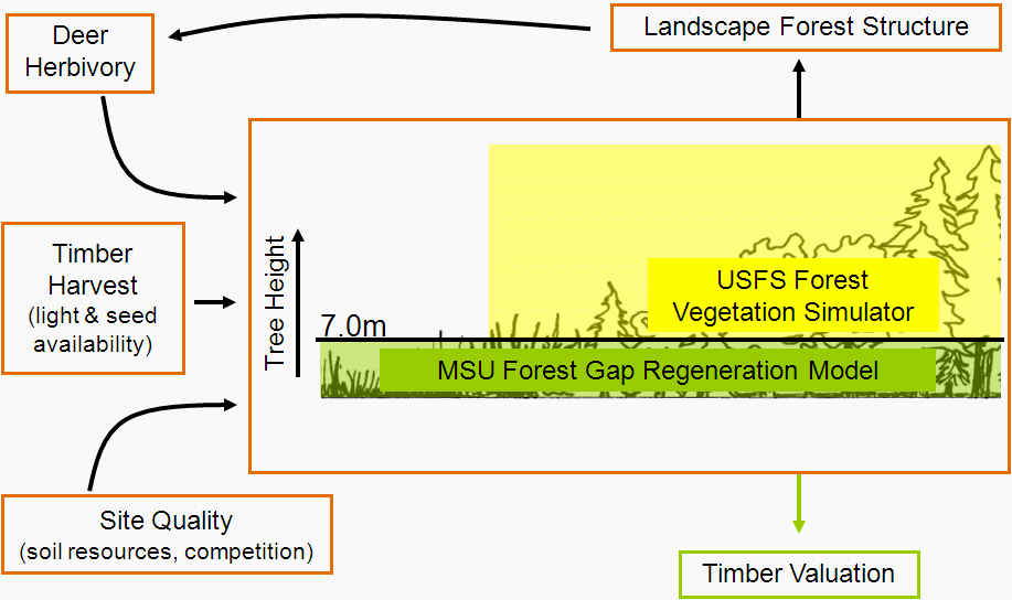
It’s taken a while but finally the model that I came to Michigan State to develop is producing what seems to be sensible output. Just recently we’ve brought all the analyses on the data that were collected in the field into a coherent whole. We’ll use this integrated model to investigate best approaches for forest and wildlife management to ensure ecological and economic sustainability. This post is a quick overview of what we’ve got at the moment and where we might take it. The image below provides a simplified view of the relationship of the primary components the model considers (a more detailed diagram is here).

The main model components I’ve been working on are the deer distribution, forest gap regeneration and tree growth and harvest sub-models. Right now we’re still in the model testing and verification stage but soon we hope to be able start putting it to use. Here’s a flow chart representing the current sequence of model execution (click for larger image):

As I’ve posted several times about the deer distribution modelling (here, here, and here for example) and because the integration of FVS with our analyses is more a technical than scientific issue, I’ll focus on the forest gap regeneration sub-model.

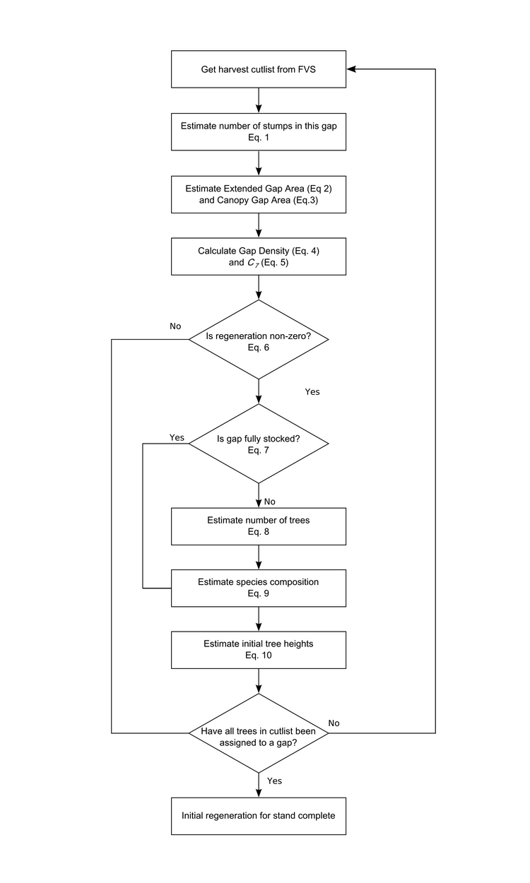
Most of the forest gap regeneration analyses used the data Megan Matonis collected during her two summers in the field (i.e., forest). During her fieldwork Megan measured gap and tree regeneration attributes such as gap size, soil and moisture regime, time since harvest, deer density, and sapling heights, density and species composition. Megan is writing up her thesis right now but we’ve also managed to find time to do some extra analyses on her data for the gap regeneration sub-model. Here’s the flow chart representing the model sequence to estimate initial regeneration in gaps created by a selection harvest in a forest stand (click for larger image):

In our gap regeneration sub-model we take a probabilistic approach to estimate the number and species of the first trees to reach 7m (this is the height at which we pass the trees to FVS to grow). The interesting equations for this are Eqs. 6 – 9 as they are responsible for estimating regeneration stocking (i.e. number of trees that regenerate) and the species composition of the regenerating trees. Through time the effects of the results of these equations will drive future forest composition and structure and the amount of standing timber available for harvest.

The probability that any trees regenerate in a gap is modelled using a generalized linear mixed model with a stand-level random intercept drawn from a normal distribution. The probability is a function of canopy gap area and deer browse category (high or low; calculated as a function of deer density in the stand).

If there are some regenerating trees in the gap, we use a logistic regression to calculate the probability that the gap contains as many (or more) trees as could fit in the gap when all the trees are 7m (and is therefore ‘fully stocked’). The probability is a function of canopy openness (calculated as a function of canopy gap area), soil moisture and nutrient conditions and deer density. If the gap is not fully stocked we sample the number of trees using from a uniform distribution.

Finally, we assign each tree to a species by estimating the relative species composition of the gap. We do this by assuming there are four possible species mixes (derived from our empirical data) and we use a logistic regression to calculate the probability that the gap has each of these four mixes. The probability of each mix is a function of soil moisture and nutrient conditions, canopy gap area, and stand-level basal area of Sugar Maple Ironwood. Currently we have parameterised the model to represent five species (Sugar Maple, Red Maple, White Ash, Black Cherry and Ironwood).

As the flow chart suggests, there is a little more to it than these three equations alone but hopefully this gives you a general idea about how we’ve approached this and what the important variables are (look out for publications in the future with all the gory details). For example, at subsequent time-steps in the simulation model we grow the regenerating trees until they reach 7m and also represent the coalescence of the canopy gaps. I haven’t integrated the economic sub-model into the program yet but that’s the next step.

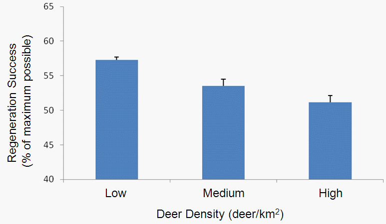
So what can we use the model for? One question we might use the model to address is, ‘how does change in the deer population influence northern hardwood regeneration, timber revenue and deer hunting value?’ For example, in one set of initial model runs I varied the deer population to test how it affects regeneration success (defined as the number of trees that regenerate as a percentage of the maximum possible). Here’s a plot that shows how regeneration success decreases with increasing deer population (as we would expect given the model structure):

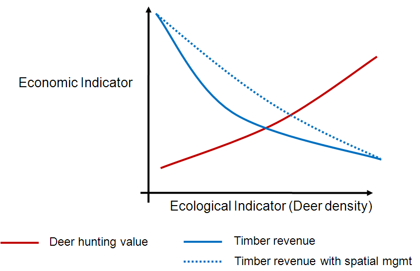
Because we are linking the ecological sub-models with economic analyses we can look at how these differences will play out through time to examine potential tradeoffs between ecological and economic values. For example, because we know (from our analyses) how the spatial arrangement of forest characteristics influences deer distribution we can estimate how different forest management approaches in different locations influences regeneration through time. The idea is that if we can reduce deer numbers in a given area immediately after timber harvest we can give trees a chance to survive and grow above the reach of deer – moving deer spatially does not necessarily mean reducing the total population (which would reduce hunting opportunities, an important part of the local economy). The outcomes may look something like this:

We plan to use our model to examine scenarios like this quantitatively. But first, I need to finish testing the model…