Around the time I wrote this blog about the National Assessment of UK Forestry and Climate Change Steering Group report I was thinking about writing a proposal to the Leverhulme Trust for an Early Career Fellowship. I found out recently that my proposal was successful and so from January 2011 I will be back at King’s College, London!
The Leverhulme Trust makes awards in support of research and education with special emphasis on original and significant research that aims to remove barriers between traditional disciplines. Their Early Career Fellowships are awarded across all disciplines and in 2010 approximately 70 were expected to be awarded to individuals to hold at universities in the UK. Given the emphasis on original, significant and cross-disciplinary research made by the Trust I looked for something that matched my research skills in coupled human and natural systems modelling but that pushed work in that area in a new direction. I thought back to the ideas about model narratives I have previously explored with David O’Sullivan and George Perry (but have not worked on since then) and Bill Cronon’s plenary address at the Royal Geographical Society in 2006 on the need for ‘sustainable narratives’. With that in mind, and given the UK Forestry and Climate change report I had been reading, I decided to make a pitch for a project that would explore how narratives from the use of models could help individuals identify how local actions transcend scales to mitigate global climate change in the context of the anticipated woodland planting that will be ongoing in the UK in future years. It proved to be a successful pitch!
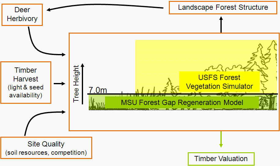
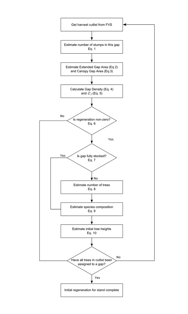
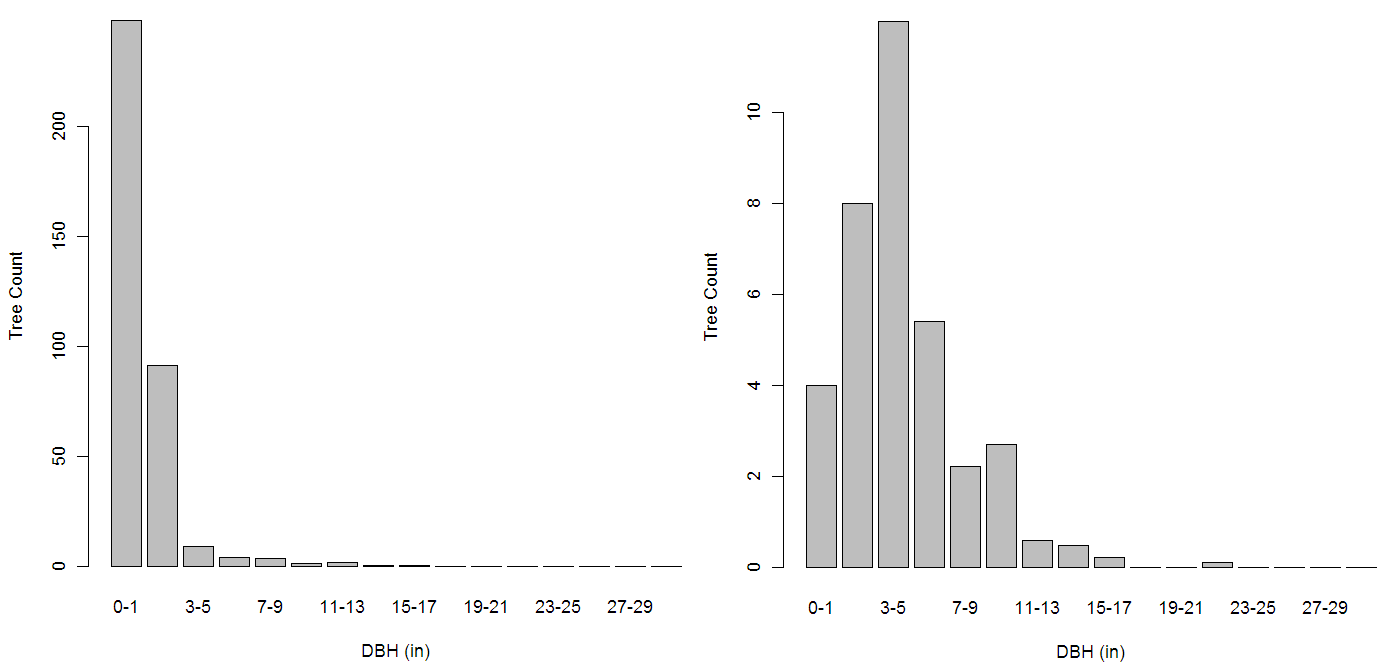
I’m sure I will blog plenty more about the project in the future, so for now I will just leave you with the proposal rationale (below). I’m looking forward to getting to work on this when I get back to London, but before that there’s plenty more things to get done on the Michigan forest landscape ecological-economic modelling.
Model narratives for climate change mitigation
The abstract, vast, and systemic narratives that dominate the issue of global climate change do little to illustrate to individuals and groups how their actions might contribute to mitigate the effects of what is often framed as a global problem (Cronon 2006). Ways to improve the ability of individuals and groups to identify how their local actions transcend scales to mitigate global climate change are needed. In this research I will explore how narratives produced from computer simulation models that represent individuals’ actions can provide people with insights into how their behaviour affects system properties at a larger scale. Although the narrative properties of simulation models have been highlighted (O’Sullivan 2004), the use of models to develop localised narratives of climate change which emphasise individual agency has yet to be explored. Confronting individuals with these narratives will also help researchers reveal important underlying, and possibly implicitly held, assumptions that influence choices and behaviour.
This research will address the following general questions:
- How can computer simulation models be better used to reveal to individuals how their local actions can contribute to global environmental issues such as Climate Change Mitigation (CCM)?
- What are the narrative properties of simulation models and how can they be exploited to help individuals find meaning about their actions as they relate to global climate change?
- By using simulation tools to spur reflection what can we learn about the factors influencing individuals’ choices and behaviour with regards CCM options?
Answering these questions will require a uniquely interdisciplinary research approach that spans the physical sciences, social sciences and humanities. Such ground-breaking, boundary-crossing work is necessary if we are to re-connect the physical sciences with the publics they intend to benefit and find solutions to large-scale and pressing environmental problems. For example, one of the key findings from a recent report by the National Assessment of UK Forestry and Climate Change Steering Group (Read et al. 2009) was that “[t]he extent to which the potential for additional [greenhouse gas] emissions abatement through tree planting is realized … will be determined in large part by economic forces and society’s attitudes rather than by scientific and technical issues alone” (p.xvii). The report also argued the need “to better understand and consider the role of different influences affecting choices and behaviour. Without the appropriate emotional, cultural or psychological disposition, information will make no difference.” (p.210). Narratives based on scientific understanding which portray how individuals can make a difference to large-scale, diffuse environmental issues will be important for fostering such a disposition. Simulation models – quantitative representations of reality which provide a means to logically examine how high-level and large-scale patterns are generated by lower-level and smaller-scale processes and events – have the potential to contribute to the construction of these narratives.
")